Engineering | Science2be

Archive | Engineering RSS feed for this section

Basics of String Theory

In this series, our primary aim is to demystify and popularize intricate mathematical structures, making them accessible to the everyday individual, both aspirational learners and mindful engineers. Even though mathematics is seen as mysterious and abstract, it is full of deep symmetry, profound truths, and beautiful things. Gaining mathematics literacy improves our ability to solve problems and creates new opportunities across many industries. A mathematically literate society is more powerful and capable of making the most use of equations and numbers to improve living standards and get a better understanding of the universe.

Introduction

The development of string theory, a cornerstone of modern theoretical physics, began in the late 1960s as a collaborative effort among several physicists, notably Gabriele Veneziano. Veneziano, in his quest to understand the strong nuclear force that binds the constituents of atomic nuclei, proposed a mathematical formula in 1968 that accurately described the scattering amplitudes of hadrons (particles like protons and neutrons) at high energies. This formula, known as the Veneziano amplitude, surprisingly mirrored the characteristics of Regge theory—a framework developed in the 1950s by Italian physicist Tullio Regge to analyze the angular momentum and properties of particles involved in scattering processes.

Regge theory introduced the concept of Regge poles, which are complex angular momenta corresponding to the resonances observed in particle physics. These poles explained the behavior of scattering amplitudes at high energies and were pivotal in understanding the dynamics of hadrons. However, the physical interpretation of Veneziano’s formula and its connection to Regge poles remained elusive until it was realized that the formula could be derived from a model where particles are not point-like but are instead envisioned as one-dimensional “strings.”

This insight led to the foundation of string theory, initially called dual resonance models, where the fundamental objects are strings whose vibrational modes correspond to different particles. The resonance phenomena, explained by Regge theory, naturally emerged from the vibrational patterns of these strings, providing a unified description of hadrons that could potentially include the graviton—the hypothetical quantum of gravity.

The initial excitement over string theory’s ability to describe the strong force waned as quantum chromodynamics (QCD) emerged as a more accurate theory for that purpose. However, string theory found new life in the 1970s and 1980s as a promising candidate for a quantum theory of gravity and a unified framework for all fundamental interactions. The introduction of supersymmetry, leading to superstring theory, further enriched the theoretical landscape, setting the stage for string theory’s evolution into a leading approach for addressing some of the most profound questions in physics.

Thus, the development of string theory, from its inception to address the issue of Regge poles and the strong nuclear force, to its current status as a potential theory of everything, illustrates a remarkable trajectory of scientific innovation and interdisciplinary collaboration.

Gabriele Veneziano made a groundbreaking contribution to theoretical physics in the late 1960s when he presented the Veneziano formula, which provided a fresh perspective on hadron scattering processes. This formula supplied the groundwork for the development of string theory in addition to fitting in with Regge theory, a framework developed to explain the angular momentum characteristics of particles. We discuss the Veneziano formula in this article, along with how it relates to Regge poles and how it makes the conceptual jump to string theory.

The Veneziano Formula: The Veneziano amplitude provided a solution to the puzzle of hadron scattering amplitudes, encapsulating the duality observed in these processes. It is expressed as:

$A(s,t) = \frac{\Gamma(-\alpha(s))\Gamma(-\alpha(t))}{\Gamma(-\alpha(s)-\alpha(t))},$

where $A(s,t)$ represents the amplitude for scattering, $\Gamma$ is the Gamma function, and $\alpha(s)$ denotes the Regge trajectory, a linear function given by:

$\alpha(s) = \alpha_0 + \alpha' s.$ Here, $\alpha_0$ is the intercept, and $\alpha'$ is the slope of the trajectory.

Let us see what it means with a concrete example.

Recall the Veneziano amplitude: $A(s,t) = \frac{\Gamma(-\alpha(s))\Gamma(-\alpha(t))}{\Gamma(-\alpha(s)-\alpha(t))}$ , where the Regge trajectory $\alpha(s)$ is linear in $s$ , the square of the total energy in the center-of-mass system: $\alpha(s) = \alpha_0 + \alpha' s$ . For this example, let’s assume values for the intercept $\alpha_0$ and the slope $\alpha'$ that are typical in discussions of string theory, though in real-world applications these would be determined by experimental data:

Let $\alpha_0 = 0.5$ , a common intercept for light mesons.
Let $\alpha' = 1\ \text{GeV}^{-2}$ , a typical value for the slope of Regge trajectories.
Example: Calculating the Amplitude for Specific $s$ and $t$ . Suppose we want to calculate the amplitude for specific values of s and t to understand the interaction at a certain energy and momentum transfer. Let’s choose:
$s = 2\ \text{GeV}^2$ (total energy squared),
$t = -1\ \text{GeV}^2$ (momentum transfer squared, negative because it’s spacelike).
First, calculate the values of $\alpha(s)$ and $\alpha(t)$ :
$\alpha(s) = 0.5 + 1 \cdot 2 = 2.5,$ $\alpha(t) = 0.5 + 1 \cdot (-1) = -0.5.$
Then, substitute these into the Veneziano amplitude: $A(2, -1) = \frac{\Gamma(-2.5)\Gamma(0.5)}{\Gamma(-2)}.$ Using the Gamma function properties and values (recall that $\Gamma(n) = (n-1)!$ for positive integers, and $\Gamma(0.5) = \sqrt{\pi}$ ): $A(2, -1) \approx \frac{\Gamma(-2.5)\sqrt{\pi}}{\Gamma(-2)}.$ The Gamma function for negative non-integer values would typically require numerical computation, but for illustrative purposes, let’s focus on the structure of the calculation rather than the exact numerical result.

A computation of the Veneziano amplitude for a given set of s and t values is only one piece of a much broader puzzle, and it may not reveal all about particle physics or string theory. Physicists can develop and improve theories that seek to explain the basic principles underlying the world by having a better understanding of the relationship between these computations and physical facts.

Connection to Regge Poles: Regge theory introduces the concept of Regge trajectories and poles, fundamental to understanding the scattering amplitudes at high energies. The Veneziano formula’s incorporation of these trajectories highlights the theory’s predictive power and its elegant mathematical structure. The linear relationship in the Veneziano formula mirrors the linear Regge trajectories observed in particle physics.

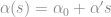
In Regge theory, the trajectory of a particle is a function that relates the angular momentum $J$ of the particle to its mass squared $m^2$ , symbolized as $J = \alpha(m^2)$ . This function is called a Regge trajectory, and it is observed to be approximately linear for many families of particles, which can be expressed as: $J = \alpha(m^2) = \alpha_0 + \alpha' m^2,$ where $\alpha_0$ (the intercept) and $\alpha'$ (the slope) are constants. The Veneziano amplitude can be written as: $A(s,t) = \frac{\Gamma(-\alpha(s))\Gamma(-\alpha(t))}{\Gamma(-\alpha(s)-\alpha(t))},$ where s and t are the Mandelstam variables representing the square of the total energy and the square of the momentum transfer in the center-of-mass frame, respectively {1}. The function $\alpha(s)$ here represents a Regge trajectory, with $s$ playing the role of $m^2$ (mass squared of the exchanged particle in the t-channel). By substituting the linear form of the Regge trajectory into the Veneziano amplitude, we explicitly see the connection: $\alpha(s) = \alpha_0 + \alpha' s$ . This implies that the resonances (or poles) in the amplitude, which correspond to physical particles, occur at values of $s$ and $t$ where $\Gamma(-\alpha(s))$ and $\Gamma(-\alpha(t))$ have poles, which is when $\alpha(s)$ and $\alpha(t)$ are non-negative integers because $\Gamma(-n)$ has poles for non-negative integers $n$ .

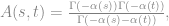
Illustration with an Example: Suppose a Regge trajectory with $\alpha_0 = 0.5$ and $\alpha' = 0.9\ \text{GeV}^{-2}$ . For a given resonance with $J = 2$ (angular momentum of the exchanged particle), we can solve for its mass squared: $2 = 0.5 + 0.9 m^2,$ , $m^2 = \frac{2 - 0.5}{0.9} \approx 1.67\ \text{GeV}^2.$ This shows how a specific point on the Regge trajectory corresponds to a resonance with a certain mass and angular momentum.

The Veneziano formula, through its incorporation of Regge trajectories, provides a powerful framework for predicting the properties of resonances in particle physics. The elegance of the formula lies in its ability to encapsulate the duality and linear relationship of Regge trajectories, offering insights into the scattering amplitudes at high energies and the spectral organization of particles.

Link to Strings: The Veneziano formula’s implications extend beyond particle physics, providing a gateway to string theory. The formula can be derived from a model in which fundamental entities are one-dimensional strings, rather than point particles. This realization unveiled a new perspective on the fabric of the universe, where the vibrational states of strings correspond to different particles, including the graviton—a hypothetical quantum of gravity naturally emerging from string theory.

Example: Prediction of the Graviton: A notable example of the Veneziano formula’s impact is its implication for quantum gravity. String theory predicts the existence of a massless spin-2 particle, identified as the graviton, through the quantization of string modes. This discovery illustrates the formula’s far-reaching consequences, bridging the gap between the strong nuclear force and the gravitational force within a unified theoretical framework. The journey from the Veneziano formula to string theory encapsulates a significant chapter in the history of theoretical physics. It illustrates how a mathematical formulation intended to describe hadron scattering led to the development of a theory that promises to unify all fundamental forces of nature, showcasing the intricate beauty and interconnectedness of the universe’s fundamental structures.

String Theory Basics, String Action (Polyakov Action):

The action for a string propagating in spacetime is given by:

$S = -\frac{1}{2\pi\alpha'} \int d\tau d\sigma (\partial_{\alpha} X^{\mu} \partial^{\alpha} X_{\mu})$

where the parameter $\alpha'$ is related to the string tension, and $X^{\mu}(\sigma,\tau)$ are the spacetime coordinates of the string. $\sigma, \tau$ are the parameters of the string worldsheet.

In string theory, the parameter α′ plays a crucial role in the dynamics of strings. It is closely related to the tension of the string, which is a fundamental property determining how the string behaves and interacts. α′ is inversely proportional to the tension of the string, T. The tension can be thought of as the energy per unit length of the string. Higher tension means the string is stiffer, as we know from classical vibrations in a guitar. Mathematically, this relationship is expressed as $T=\frac{1}{2 \pi \alpha '}$ .

The value of α′ affects the mass spectrum of the particles represented by string modes. It determines the scale at which stringy effects become significant. Typically, it’s set to a very small value, ensuring that stringy behavior is evident only at very high energies, far beyond the reach of current particle accelerators.

Example with a Known Particle:

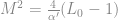
Quantization: By quantizing this action (applying quantum mechanics to string theory), we obtain a spectrum of possible vibrational states of the string. Each state can be interpreted as a different particle. Calculating Particle Properties, Mass Spectrum: The mass of the vibrational modes is determined by the level of excitation of the string. For a closed string, the mass formula in the simplest case is given by: $M^2 = \frac{2}{\alpha'}(N-1)$ where $N$ is the number operator, representing the level of string excitation.

Spin and Other Quantum Numbers: The type of vibration (how the string vibrates in different dimensions) determines the spin and other quantum numbers of the particles. For instance, a string vibrating in a particular mode might correspond to a particle with spin-1, like a photon.

Tachyons and Stability: Early models of string theory predicted particles with imaginary mass, known as tachyons, indicating an instability in the theory. This led to the development of superstring theory, which includes fermions and supersymmetry, to address these issues.

General Relativity (Higher-Dimensional Metrics): In higher-dimensional general relativity, the spacetime metric extends beyond four dimensions. For instance, in 5D Kaluza-Klein theory, the metric tensor $g_{AB}$ (where $A, B$ run from 0 to 4) combines the 4D spacetime metric with an extra dimension, potentially unifying gravity and electromagnetism.

Topological Quantum Field Theory (TQFT): In TQFT, one often encounters algebraic structures like tensor categories. An example is the partition function $Z$ which assigns a complex number to a manifold $M$ :
$Z(M) = \int \mathcal{D}\phi e^{iS[\phi]}$ where $S[\phi]$ is the action functional of the field $\phi$ over the manifold $M$ . In higher dimensions, these structures become more complex and are often studied using higher categorical algebra.

Condensed Matter Physics (Topological Insulators): In topological insulators, the Chern number, an integer describing the topology of the band structure, plays a crucial role. It is given by an integral over the Brillouin zone:
$C_n = \frac{1}{2\pi i} \int_{BZ} d^2k \, \text{Tr} \left( F_{12}(k) \right)$
where $F_{12}(k)$ is the Berry curvature in momentum space. In higher-dimensional systems, these integrals extend over more complex manifolds.

String Theory Quantization and Mass Spectrum

The process of deriving the mass spectrum in string theory from the Polyakov action involves several steps, outlined as follows:

Mode Expansion: The string’s spacetime coordinates, $X^\mu(\sigma, \tau)$ , are expanded in terms of mode functions.

Canonical Quantization: Apply quantum mechanics principles, promoting classical fields to quantum operators and imposing commutation relations.

Virasoro Operators: From the quantization, we obtain Virasoro operators $L_m$ , which are central to string theory. These operators are constructed from the energy-momentum tensor derived from the Polyakov action.

The Virasoro operators play a pivotal role in the quantization of string theory, providing an algebraic structure essential for the theory’s consistency. They emerge from the energy-momentum tensor derived from the Polyakov action, encapsulating the dynamics of strings in spacetime.

-Virasoro Operators: The Virasoro algebra consists of an infinite set of operators $L_m$ and their antiholomorphic counterparts $\bar{L}_m$ , where $(m)$ is an integer. These operators satisfy the following commutation relations:

$[L_m, L_n] = (m - n)L_{m+n} + \frac{c}{12}m(m^2 - 1)\delta_{m+n,0},$

$[\bar{L}_m, \bar{L}_n] = (m - n)\bar{L}_{m+n} + \frac{\bar{c}}{12}m(m^2 - 1)\delta_{m+n,0},$

where $c$ and $\bar{c}$ are the central charges, and $\delta_{m+n,0}$ is the Kronecker delta function.

-Physical State Conditions: A state $|\psi\rangle$ in string theory is considered physical if it satisfies the Virasoro constraints:

$(L_m - \delta_{m,0})|\psi\rangle = 0, \quad \text{for } m \geq 0,$

$(\bar{L}_m - \delta_{m,0})|\psi\rangle = 0, \quad \text{for } m \geq 0.$

-These conditions ensure the elimination of negative norm states and the proper quantization of the string’s energy levels.

Example: Massless Scalar Field: To illustrate the application of Virasoro operators, consider a bosonic string in flat spacetime. The mode expansion of $X^\mu$ leads to quantized oscillatory modes, and the Virasoro operators are expressed as:

$L_m = \frac{1}{2} \sum_{n=-\infty}^{\infty} :\alpha_{m-n} \cdot \alpha_n:$ ,

where $\alpha_n^\mu$ are the oscillator modes, and the normal ordering is denoted by $:.:$ . For a massless scalar field, consider the state created by acting on the vacuum with $\alpha_{-1}^\mu$

$|\psi\rangle = \alpha_{-1}^\mu |0;k\rangle.$

This state represents a massless particle, satisfying the physical state conditions, including the crucial $L_1$ constraint: $k_\mu \alpha^\mu_1 |0;k\rangle = 0,$ indicating that $k^2 = 0$ , where $k$ is the momentum of the state, identifying it as a massless scalar field in the spectrum of string theory. The Virasoro operators are instrumental in defining the physical states of string theory, ensuring the theory’s consistency by eliminating unphysical states and determining the properties of the particles in the string spectrum.

The plot above illustrates a Regge trajectory, which is a linear relationship between the angular momentum J and the mass squared (s) of particles. This concept is pivotal in understanding the dynamics of hadrons in particle physics. Each point on the trajectory represents a different vibrational state of a string, corresponding to different particles (e.g., mesons, baryons, tetraquarks, pentaquarks) with increasing mass and angular momentum. This visualization encapsulates the essence of how string theory’s vibrational modes relate to the physical properties of particles, echoing the foundational principles laid out by the Veneziano formula and Regge theory.

Level Matching Condition: For closed strings, the left-moving and right-moving modes of vibration must be equal, leading to a level matching condition $L_0 = \bar{L}_0$ .

Mass Formula: The mass-squared operator in string theory is related to these Virasoro operators. For a closed string, the mass-squared is given by:
$M^2 = \frac{4}{\alpha'} (L_0 - 1)$
for the left-moving modes and similarly for the right-moving modes with $\bar{L}_0$ .

But the main interest for this text is: can string theory be helpful for the society, for anyone beyond the limited and rarefied atmosphere of the savants? The answer is, yes.

The formalism and ideas of string theory, while fundamentally rooted in the quest to understand the universe’s smallest constituents and forces, also inspire innovative approaches across various fields, including medicine, engineering, and finance. Here are some specific examples where the formalism and ideas of string theory might find application outside of pure physics:

Medicine: Understanding Genetic Diseases

Genomic Sequences as Strings: In bioinformatics, sequences of DNA and RNA can be thought of as strings of nucleotides. Analogous to how string theory considers vibrating strings as fundamental elements that compose particles, genomic sequences can be analyzed using string theory formalisms to understand genetic variations and mutations. This perspective can aid in the development of gene therapies and precision medicine by modeling the interactions between different genetic elements in complex diseases.

Engineering: Design of Meta-materials

Vibration and Resonance in Materials: String theory’s focus on vibration and resonance has parallels in the engineering of meta-materials, which are artificial materials engineered to have properties not found in naturally occurring materials. By applying the concepts of vibration modes from string theory, engineers can design meta-materials with unique electromagnetic or acoustic properties, useful in developing cloaking devices, superlenses, and highly efficient energy transmission systems.

Finance: Modeling Market Dynamics

Complex Systems and Entanglement: String theory’s treatment of entangled states, where particles remain connected across vast distances, offers a metaphorical framework for understanding complex financial systems where global markets are deeply interconnected. By borrowing mathematical tools from string theory, financial analysts could model market dynamics under the lens of entanglement, potentially offering new insights into how information and trends propagate through global financial networks, affecting asset prices and market stability.

Cross-disciplinary: Network Theory and Machine Learning

Topology and Connectivity: The study of Calabi-Yau manifolds and other complex topologies in string theory can inspire new algorithms in network theory and machine learning. Understanding how these shapes encode information about extra dimensions could parallel how information is structured and flows in complex networks, leading to innovative ways to analyze connectivity patterns in social networks, the brain, or the internet.

Quantum Computing

Quantum Information Processing: String theory’s exploration of higher-dimensional spaces and quantum gravity might inform the development of quantum computing algorithms by providing insights into the nature of quantum entanglement and coherence. As quantum computing seeks to harness these properties for computing power, insights from string theory could guide the design of more efficient quantum algorithms and error correction methods, with applications ranging from cryptography to drug discovery.

While the direct application of string theory’s formalism to these fields may require a creative leap, the underlying mathematical tools and conceptual frameworks offer a rich source of inspiration. The analogies and insights derived from string theory can stimulate innovative approaches to longstanding problems, driving advancements in technology, finance, and healthcare.

Just look at these references to imagine the span of applications of string theory concepts in fields outside of traditional physics:

Data Science Applications to String Theory by Fabian Ruehle (2020) discusses how machine learning and data science techniques can be applied to string theory, including example codes. These approaches could potentially be adapted for use in medicine, engineering, and finance .https://www.sciencedirect.com/science/article/pii/S0370157319303072
Nonlocality in String Theory by G. Calcagni and L. Modesto (2013) explores the concept of nonlocality in string theory, which could have implications for understanding complex systems in engineering and finance. https://iopscience.iop.org/article/10.1088/1751-8113/47/35/355402/pdf
String Field Theory by Harold Erbin provides an introduction to string field theory, which as a field theory, offers a constructive formulation of string theory. This formalism could inspire new computational models in various disciplines. https://arxiv.org/abs/2301.01686
String Theory and Particle Physics: An Introduction to String Phenomenology by L. Ibáñez and Á. Uranga (2011) focuses on how string theory is connected to the real world of particle physics, providing models of physics beyond the Standard Model. The methodologies discussed could find applications in computational biology and complex systems engineering. https://www.cambridge.org/core/books/string-theory-and-particle-physics/7D005A97DA657F6675C2A62E449FC62E
Introduction to String Theory by Samarth Parekh (2022) offers an overview of the basic concepts of string theory, including its implications for quantum field theory, gravitational physics, and the nature of spacetime. These concepts could potentially influence advanced computational techniques in medicine and finance. https://papers.ssrn.com/sol3/papers.cfm?abstract_id=4009963
Focus Issue on String Cosmology by V. Balasubramanian and P. Moniz (2011) appraises recent applications of string-theoretic and string-inspired ideas to cosmology. The discussion on alternative models and dynamics could inspire novel approaches in data analysis and predictive modeling in finance. https://iopscience.iop.org/article/10.1088/0264-9381/28/20/200301

POSTSCRIPT:

The strong nuclear force appears to be described by Leonhard Euler’s beta function, as Gabrielle Veneziano inadvertently found in 1968. Because it is a function of the binomiale distribution, the beta function gets its name. As previously mentioned, it may be connected to the gamma function. In 1969, Veneziano discovered that Euler’s beta function was a suitable option when searching for a function that satisfies the basic postulates for the scattering amplitudes of elementary particles in strong contact. String theory was launched by this initial step, despite the fact that Veneziano was searching for a theory of strong interactions.

According to string theory, the cosmos is made up of vibrating energy filaments, or strings, as it presents us with a new understanding of the universe. The presence of additional physical things known as branes is also predicted by this scientific theory. String theory is a quantum field theory that describes the existence of particles and the generation of forces based on the compactification—the process of condensing hidden dimensions into extremely small sizes—at the level of high-energy theoretical physics.

The hypothesis was created in 1968 in an effort to explain hadron behaviour, but it was quickly shelved until the middle of the 1980s since it required more hidden dimensions. It developed into the M-theory, a more complex theory, in the 1990s [FN1]. Not only does string theory bring all particles together, but it also brings together the forces that govern their interactions. The electromagnetic field is a force that kind of spreads over space, enabling object interaction, and it fits the quantum theory rather well. Gravity doesn’t, though. And why? primarily because space is warped by gravity [FN2].

Additional References:

[FN1] The other leading alternative is known as loop quantum gravity. According to this theory space consists of not ordinary atoms, but extremely small chunks of space (like knots in a carpet).

[FN2] Quantum theory of gravity try to handle with this.

{1} The variables s and t are Mandelstam variables, key components in the description of particle collisions. They are defined in the context of a scattering process involving two incoming particles and two outgoing particles.

The Mandelstam variable s is defined as the square of the total energy in the center-of-mass frame. It reflects the overall energy available for the interaction. In mathematical terms, for particles with four-momenta p1 and p2, it’s defined as $s=(p1+p2)^2$ . It gives an indication of the energy level at which the scattering process occurs.
The Mandelstam variable t, on the other hand, represents the square of the momentum transfer between the incoming and outgoing particles. It’s defined as $t=(p1-p3)^2$ , where p3 is the four-momentum of one of the outgoing particles. This variable measures how much the direction of motion of the particles has changed due to the scattering process.

The function α(s) and α(t) are Regge trajectories, which relate the spin of a particle to its mass squared, essentially describing how the properties of exchanged particles in the interaction vary with s and t. These trajectories are central in reggeon field theory, a framework used before QCD to describe the strong interaction at high energies.

The Veneziano amplitude thus combines these elements to predict the likelihood (amplitude) of various outcomes of particle collisions at different energy levels (s) and angles (t). Its form, invoking the Gamma function, ensures the amplitude has poles at integer values of −α(s) and −α(t), corresponding to the masses of the resonances involved in the scattering process. This was an attempt to explain the pattern of hadron masses and their interactions in the era before quarks and gluons were established as the fundamental constituents of hadrons.

Acknowledgment: Part of this post was based on the course materials provided by MIT’s course, “String Theory for Undergraduates” available in Spring 2007. More information can be found at: https://ocw.mit.edu/courses/8-251-string-theory-for-undergraduates-spring-2007/

Comments Leave a Comment
Categories Academia, Education and Science, Engineering, Medicine, Quantum computers, String Theory

The Palatini Formalism and The Ashtekar Variables – An Engineered Approach

26 Jan

Two significant people in the fascinating topic of mathematical physics are Abhay Ashtekar and Attilio Palatini. The dynamics of general relativity were subtly revised in the early 20th century by the Italian scientist Attilio Palatini. Many years later, the Indian theoretical physicist Abhay Ashtekar cleared a route for revolution in the field of quantum gravity by introducing additional variables that improved the tractability of the quantum description of gravity. The fundamental concepts in deciphering the innermost workings of the universe are the Palatini Formalism and the Ashtekar Variables. Scholars understand their great significance, but we hope to shed light on these complex subjects for hobbyists, engineers, and aspiring physicists. The following sources are must-read for anyone interested in learning more about these curious topics:

Rovelli, C. (2004). Quantum Gravity. Cambridge University Press.
Thiemann, T. (2007). Modern Canonical Quantum General Relativity. Cambridge University Press.
Ashtekar, A., & Lewandowski, J. (2004). Background independent quantum gravity: A status report. Classical and Quantum Gravity.
Palatini, A. (1919). Deduzione invariantiva delle equazioni gravitazionali dal principio di Hamilton. Rendiconti del Circolo Matematico di Palermo.
Pullin, J., & Gambini, R. (2011). A First Course in Loop Quantum Gravity. Oxford University Press.

Join us as we try to uncover some of the secrets hidden behind these mathematical marvels, offering a unique viewpoint that helps us to better understand the intricate details of the universe.

The Palatini approach offers a different take on the Einstein-Hilbert action, reformulating it in terms of a connection and a frame field rather than the metric. This differentiation allows for a different means of variation, which leads to first-order field equations rather than the second-order ones derived from the Einstein-Hilbert action.

In the standard formulation of general relativity, the action is described in terms of the metric $g_{\mu\nu}$ . The Einstein-Hilbert action is given by:
$\displaystyle S_{EH} = \int d^4x \sqrt{-g} R$
where $R$ is the Ricci scalar and $\sqrt{-g}$ is the square root of the determinant of the metric tensor.

In the Palatini formulation, the action is written as a function of a connection $\Gamma^\lambda_{\mu\nu}$ and a “frame field” or “tetrad” $e^a_\mu$ . The action is expressed as:
$S_{Palatini} = \int d^4x \sqrt{-\text{det}(e)} R(e, \Gamma)$
Here, $R(e, \Gamma)$ is the Ricci scalar but now expressed in terms of the connection and the tetrad, and $\sqrt{-\text{det}(e)}$ is the square root of the determinant of the tetrad.

Fig. 1 – Fibre Visualisation in Space. This image, which was produced with the Deep Image Generator, shows a complicated web of fibres with recursive patterns and fractal geometry. The generator simulates the complex and multidimensional nature of fibre structures in a spatial environment by using algorithmic techniques based on differential geometry and topology optimisation. The graphic displays the complex weaving and bundling that characterise fibrous networks, emphasising the interaction between linear and nonlinear components.

Here, the Ricci scalar $R(e,\Gamma)$ in the Palatini formulation is a function of both the tetrad (or frame field) $e^a_{\mu}$ and the connection $\Gamma^{\lambda}_{\mu\nu}$ . The actual functional form can be a bit involved, but we can summarize it as:

Define the curvature tensor using the connection:

$R^{\sigma}_{\mu \nu \rho}(\Gamma)=\partial_{\mu} \Gamma^{\sigma}_{\nu \rho} -\partial_{\nu}\Gamma^{\sigma}_{\mu\rho}+\Gamma^{\sigma}_{\mu\lambda} \Gamma^{\lambda}{\nu\rho}-\Gamma^{\sigma}{\nu\lambda} \Gamma^{\lambda}_{\mu\rho}$

Define the Ricci tensor in terms of this curvature tensor:
$R_{\mu\nu}(\Gamma) = R^{\rho}_{\mu\nu\rho}(\Gamma)$

Define the metric using the tetrad:
$g_{\mu\nu} = e_{\mu}^a e_{\nu}^a$

And then define the Ricci scalar:
$R(e,\Gamma) = g^{\mu\nu} R_{\mu\nu}(\Gamma)$

Given this, the Palatini action becomes a functional of both $e^a_{\mu}$ and $\Gamma^{\lambda}_{\mu\nu}$ .

When varying the action with respect to $\Gamma^{\lambda}_{\mu\nu}$ , we enforce the condition that the connection is metric-compatible, meaning it preserves the metric under parallel transport. This yields the usual Levi-Civita connection (Christoffel symbols) in terms of the metric defined by the tetrad. On the other hand, varying with respect to $e^a_{\mu}$ yields Einstein’s field equations with the energy-momentum tensor on the right side.

In a nutshell:

Varying with respect to the connection $\Gamma^{\lambda}{\mu\nu}$ gives:

$\frac{\delta S{\text{Palatini}}}{\delta \Gamma^{\lambda}_{\mu\nu}} = 0$
This equation yields the connection as the Levi-Civita connection (in terms of the metric).

Varying with respect to the tetrad $e^a_\mu$ gives:
$\frac{\delta S_{\text{Palatini}}}{\delta e^a_\mu} = 0$ .
This equation produces Einstein’s field equations.

The critical distinction is that in the Palatini formalism, the connection and the metric (or tetrad) are treated as independent variables, whereas in the standard Einstein-Hilbert action, the connection is derived solely from the metric, making them dependent on one another.

The Palatini formalism, as mentioned before, is an approach to deriving the field equations of general relativity by treating the metric (or tetrad) and the connection as independent variables, rather than the more traditional approach where the connection (Christoffel symbols) is derived from the metric.

Consider the Palatini formalism, where the metric and the connection are treated as independent entities. This separation of structures can remind us of the principle of least action, where dynamics are derived from an action principle. Let’s try to take inspiration from this in the context of electromagnetism.

Example: A Palatini-inspired Approach to Electromagnetism

Suppose we’re looking to derive the equations of electromagnetism using a variational principle, but instead of the standard action, we’ll treat the electric and magnetic fields, $(\vec{E}) and (\vec{B})$ , as separate independent entities rather than derivatives of a potential. This is a bit contrived and is more of a pedagogical exercise than a real physics one, but it serves as an illustrative example. The steps to be done are:

Construct an Action: We could build an action, (S), that’s a functional of $(\vec{E}), (\vec{B})$ , and other required potentials. For the sake of this example, suppose:
$S[\vec{E},\vec{B}] = \int d^3 x dt \left( \vec{E} \cdot \frac{\partial \vec{A}}{\partial t} + \vec{B} \cdot (\nabla \times \vec{A}) - \frac{1}{2} (\vec{E}^2 + \vec{B}^2) \right)$
where $(\vec{A})$ is the vector potential.

Variation with Respect to Fields: By treating $(\vec{E})$ and $(\vec{B})$ as independent (akin to treating metric and connection as independent in the Palatini formalism), we would derive equations of motion for $(\vec{E})$ and $(\vec{B})$ by varying the action with respect to them.

Derive Equations: By performing the variations, one would obtain equations linking the fields $(\vec{E}) and (\vec{B})$ to the potentials and currents, similar to Maxwell’s equations.

This is merely an illustration of an alternative approach that we could use to derive Maxwell’s equations, but it also shows how a Palatini-like strategy (considering normally dependent quantities as independent) can be used in contexts other than general relativity. This is a different approach to the problem and would help students better comprehend variational principles and the Palatini method, but it wouldn’t necessarily offer any new insights about electromagnetism.

When it comes to handling the complexity of gravity, particularly when integrating it with quantum physics, methods like the Palatini or Ashtekar formalism truly dazzle. Applying them to easier situations is similar to trying to crack a nut with a sledgehammer; it’s feasible but it’s not always the most effective or insightful approach.

To obtain equations like Maxwell’s equations, we will step through a variant of the hypothetical action. Be aware that this is an unconventional method for teaching; the goal is not to learn new things about electromagnetism, but to illustrate the technique.

Let’s start with the action:
$S[E,B] = \int d^3 x dt \left( \vec{E} \cdot \frac{\partial \vec{A}}{\partial t} + \vec{B} \cdot (\nabla \times \vec{A}) - \frac{1}{2} (\vec{E}^2 + \vec{B}^2) \right)$

Variation with respect to $(\vec{E})$ :
The variation of the action with respect to $(\vec{E})$ is:
$\frac{\delta S}{\delta \vec{E}} = \frac{\partial \vec{A}}{\partial t} - \vec{E}$
Setting this to zero gives:
$\vec{E} = \frac{\partial \vec{A}}{\partial t}$
which is consistent with the usual relation between the electric field and the vector potential.

Variation with respect to $(\vec{B})$ :
The variation of the action with respect to $(\vec{B})$ is:
$\frac{\delta S}{\delta \vec{B}} = \nabla \times \vec{A} - \vec{B}$
Setting this to zero gives:
$\vec{B} = \nabla \times \vec{A}$ .
This is the standard relation between the magnetic field and the vector potential.

To complete the analogy with Maxwell’s equations, we would also have to include the scalar potential $(\phi)$ and introduce sources (charge and current densities) to the action. That would provide us with equations relating the divergence of $(\vec{E})$ and $(\vec{B})$ to the charge density and showing that the divergence of $(\vec{B})$ is zero.

While our contrived action correctly reproduces two of Maxwell’s equations when varied with respect to (\vec{E}) and (\vec{B}), it is important to remember that in actual electromagnetism, (\vec{E}) and (\vec{B}) are derived from potentials and are not independent entities. The true action for electromagnetism involves the electromagnetic field tensor and its dual, from which all of Maxwell’s equations can be derived.

This exercise was mainly to show the use of the Palatini-style approach in a simpler context and to see how variational principles work.

Comments Leave a Comment
Categories Academia, Calculus of Variations, DIY laboratories, Economic progress, Education and Science, Electromagnetic field, Engineering, General Relativity, Quantum Loop Gravity

Finite Differences vs Finite Volumes: An Introduction with the example of the Plasma Plume Continuity Simulation

16 Oct

Introduction:

In the complex subject of plasma propulsion, understanding the behavior of ejected plasma plumes is paramount. These plumes, consisting of swift-moving ions and electrons, present complex interactions, especially when they encounter external magnetic fields. Such complexities necessitate the use of computational models that can accurately depict the electron density profiles. One commonly adopted approach is the Finite Difference (FD) method, which, while straightforward, may sometimes falter in representing these profiles accurately, especially on coarser grids. On the other hand, the Finite Volumes (FV) method, with its robust focus on conservation, offers an alternative that promises greater accuracy. This article delves into these methods, comparing their effectiveness and illustrating their application with a 1D electron density profile.

In computational physics, the choice of numerical method can make all the difference. This article delves into the comparison between Finite Differences (FD) and Finite Volumes (FV) methods, exploring their application to the continuity of plasma plumes.

The Context: Plasma Plumes in Space Propulsion

Electric thrusters for space propulsion eject plasma plumes — clouds of ions and electrons moving at hypersonic speeds. These plumes can interact with external magnetic fields, complicating their behavior. Formally, if n is our electron density, it satisfies the continuity equation: ∂n/∂t+∇⋅(nv)=0 where v is the velocity field.

Finite Differences (FD) Method:

FD discretizes differential equations by approximating derivatives using differences. For instance, the first derivative can be represented as df/dx≈(f(x+h)−f(x))/h When applied to our continuity equation on a grid, FD might lead to errors, especially if ℎ (the grid spacing) is not sufficiently small.

Example: Consider a 1D electron density profile given by: n(x)=sin(x) When we use a coarse grid, the FD method might misrepresent the profile, leading to inaccuracies in the simulation.

Finite Volumes (FV) Method:

FV focuses on conservation. The domain is divided into small volumes, and the equation is integrated over each volume. Our continuity equation becomes: ∫_V ∂n/∂t dV+∮_S nv⋅dS=0 Here, V is the control volume and S its boundary. FV ensures that whatever enters or leaves a volume is conserved, offering better accuracy for phenomena like plasma plumes.

Example: Revisiting our 1D electron density n(x)=sin(x) the FV method, even with a coarse grid, would capture the essence of the density profile without major continuity errors.

Comparison in Plasma Plume Simulation:

While FD’s simplicity is alluring, it can struggle with continuity equations in coarser grids. FV, with its focus on conservation, tends to provide more consistent results, especially when accuracy over larger domains is crucial.

Conclusion:

Both FD and FV have their niches, but when it comes to plasma plume continuity, where conservation is paramount, FV often outshines FD. With accurate simulations being pivotal for space propulsion research, understanding the strengths and weaknesses of these methods is paramount.

# Import necessary libraries
import numpy as np
import matplotlib.pyplot as plt

# Define parameters
L = 10.0  # Length of the domain
nx = 100  # Number of grid points
dx = L/nx  # Grid spacing
dt = 0.01  # Time step
v = 1.0  # Particle velocity
t_end = 0.5  # End time

# Initial condition: Gaussian profile for density
x = np.linspace(0, L, nx)
n0 = np.exp(-((x - L/4)**2) / 2)
n_fd = np.copy(n0)
n_fv = np.copy(n0)

# FD method
for t in np.arange(0, t_end, dt):
    n_fd[:-1] = n_fd[:-1] - v*dt/dx * (n_fd[1:] - n_fd[:-1])

# FV method
for t in np.arange(0, t_end, dt):
    flux = v * 0.5 * (n_fv[1:] + n_fv[:-1])
    n_fv[1:-1] += (flux[:-1] - flux[1:]) * dt/dx

# Plot results
plt.figure(figsize=(10, 6))
plt.plot(x, n0, label="Initial")
plt.plot(x, n_fd, label="Finite Difference")
plt.plot(x, n_fv, label="Finite Volume")
plt.legend()
plt.title("Evolution of Plasma Plume Density")
plt.xlabel("x")
plt.ylabel("Density, n")
plt.show()